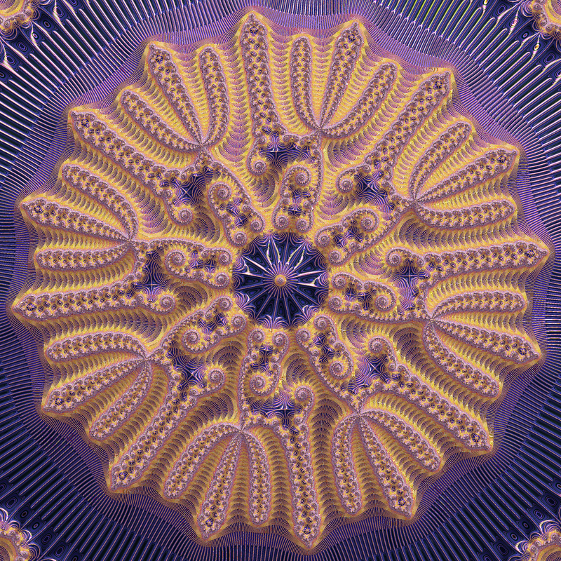
09 - A deeper DEM example

This example shows how to create a color layer which displays a distance estimation from the Mandelbrot (power 2) fractal.

The location, at 1.8e-157, is well below the separation power of double, pertubation theory must be used. This location, “Dinkidau flake”, is a common test for numerical reliability.

Reference: fractalshades.models.Perturbation_mandelbrot

import os
import numpy as np

import fractalshades as fs
import fractalshades.models as fsm
import fractalshades.settings as settings
import fractalshades.colors as fscolors
import fractalshades.projection


from fractalshades.postproc import (
    Postproc_batch,
    DEM_pp,
    Continuous_iter_pp,
    Raw_pp,
    DEM_normal_pp,
)
from fractalshades.colors.layers import (
    Color_layer,
    Bool_layer,
    Normal_map_layer,
    Virtual_layer,
    Blinn_lighting
)

def plot(directory):
    """
    Example plot of distance estimation method
    """
    settings.enable_multithreading = True
    # A simple showcase using perturbation technique
    precision = 165
    nx = 2400
    x = '-1.99996619445037030418434688506350579675531241540724851511761922944801584242342684381376129778868913812287046406560949864353810575744772166485672496092803920095332'
    y = '-0.00000000000000000000000000000000030013824367909383240724973039775924987346831190773335270174257280120474975614823581185647299288414075519224186504978181625478529'
    dx = '1.7e-157'

    colormap = fscolors.cmap_register["valensole"]

    f = fsm.Perturbation_mandelbrot(directory)
    f.zoom(precision=precision,
            x=x,
            y=y,
            dx=dx,
            nx=nx,
            xy_ratio=1.0,
            theta_deg=0.,
            projection=fs.projection.Cartesian()
    )

    f.calc_std_div(
            calc_name="div",
            subset=None,
            max_iter=1000000,
            M_divergence=1.e3,
            epsilon_stationnary=1.e-3,
            BLA_eps=1.e-8,
            interior_detect=False
    )


    # Plot the image
    pp = Postproc_batch(f, "div")
    pp.add_postproc("potential", Continuous_iter_pp())
    pp.add_postproc("DEM", DEM_pp())
    pp.add_postproc("interior", Raw_pp("stop_reason", func="x != 1."))
    pp.add_postproc("DEM_map", DEM_normal_pp(kind="potential"))

    plotter = fs.Fractal_plotter(pp, final_render=False, supersampling="2x2")
    plotter.add_layer(Bool_layer("interior", output=False))
    plotter.add_layer(Normal_map_layer("DEM_map", max_slope=35, output=False))
    plotter.add_layer(Virtual_layer("potential", func=None, output=False))
    plotter.add_layer(Color_layer(
            "DEM",
            func="np.log(x)",
            colormap=colormap,
            probes_z=[0., 5.0],
            output=True
    ))
    plotter["DEM"].set_mask(
            plotter["interior"],
            mask_color=(0., 0., 0.)
    )
    plotter["DEM_map"].set_mask(plotter["interior"], mask_color=(0., 0., 0.))


    # This is where we define the lighting (here 2 light sources)
    # and apply the shading
    light = Blinn_lighting(0.35, np.array([1., 1., 1.]))
    light.add_light_source(
        k_diffuse=0.0,
        k_specular=600.,
        shininess=200.,
        polar_angle=75.,
        azimuth_angle=5.,
        color=np.array([0.9, 0.9, 0.2]))
    light.add_light_source(
        k_diffuse=1.9,
        k_specular=0.,
        shininess=400.,
        polar_angle=75.,
        azimuth_angle=30.,
        color=np.array([1., 1., 1.]))
    plotter["DEM"].shade(plotter["DEM_map"], light)

    plotter.plot()

if __name__ == "__main__":
    # Some magic to get the directory for plotting: with a name that matches
    # the file or a temporary dir if we are building the documentation
    try:
        realpath = os.path.realpath(__file__)
        plot_dir = os.path.splitext(realpath)[0]
        plot(plot_dir)
    except NameError:
        import tempfile
        with tempfile.TemporaryDirectory() as plot_dir:
            fs.utils.exec_no_output(plot, plot_dir)